Table of Contents >> Show >> Hide
If statistics had a PR team, the confidence interval would be its least flashy but most useful employee. It does not do fireworks. It does not wear sunglasses indoors. What it does do is tell you how precise your estimate probably is. And that matters whether you are reading a medical study, running an A/B test, analyzing survey data, or trying to sound smarter in a meeting without becoming that person who says “the data speaks for itself.”
In plain English, a confidence interval gives you a range of likely values for a population parameter based on your sample data. Instead of saying, “The average is 72,” you say, “The average is probably somewhere between 67.9 and 76.1.” That second version is more honest, more informative, and far less likely to get roasted by a stats professor.
This guide breaks the process into six clear steps. You will learn the core confidence interval formula, when to use a z-score versus a t-score, how to calculate margin of error, and how to interpret the final interval without committing one of the classic statistics sins. We will also walk through examples for both a sample mean and a sample proportion so the concept sticks.
What Is a Confidence Interval?
A confidence interval is a range built around a sample statistic, such as a sample mean or sample proportion. That range is designed to capture the true population value at a chosen confidence level, usually 90%, 95%, or 99%.
The general structure looks like this:
confidence interval = point estimate ± margin of error
The point estimate is your best single-number guess from the sample. The margin of error is the “wiggle room” added on each side. Bigger wiggle room means less precision. Smaller wiggle room means a tighter estimate. This is why a narrow confidence interval usually feels more satisfying. It is the statistical version of getting a delivery window of “between 2:00 and 2:15” instead of “sometime this week.”
Why Confidence Intervals Matter
Confidence intervals matter because single estimates can be misleading. A sample is only a slice of the full population, so uncertainty is baked into the process. Confidence intervals quantify that uncertainty.
They are also more useful than a lonely p-value in many real-world situations because they show both direction and precision. A p-value can tell you something is statistically significant. A confidence interval shows whether the effect is tiny, huge, plausible, or all over the map like a squirrel on espresso.
How to Calculate Confidence Interval: 6 Steps
Step 1: Identify the Parameter and Your Point Estimate
Start by figuring out what you are estimating. Is it a population mean, a population proportion, a difference between groups, or something else? For most beginners, the two common cases are:
- Population mean, estimated by the sample mean
x̄ - Population proportion, estimated by the sample proportion
p̂
Examples:
- If 25 students have an average test score of 72, then
x̄ = 72 - If 240 out of 400 customers prefer option A, then
p̂ = 240 / 400 = 0.60
Your point estimate is the center of the confidence interval. Everything else in the calculation is basically about deciding how wide the interval should be.
Step 2: Choose a Confidence Level
The confidence level tells you how often the method would capture the true parameter if you repeated the sampling process many times. The most common choices are:
- 90%: narrower interval, less confidence
- 95%: common default, good balance
- 99%: wider interval, more confidence
Here is the trade-off: higher confidence means a wider interval. You get more coverage, but less precision. So if someone demands a super-tight interval and a super-high confidence level at the same time, that person is asking statistics to do yoga and powerlifting simultaneously.
Step 3: Calculate the Standard Error
The standard error measures how much your sample statistic would vary from sample to sample. It is the engine under the confidence interval hood.
For a sample mean:
SE = s / √n
Where:
s= sample standard deviationn= sample size
For a sample proportion:
SE = √[ p̂(1 - p̂) / n ]
Where:
p̂= sample proportionn= sample size
Important note: larger samples usually give you a smaller standard error, which leads to a narrower confidence interval. This is one reason sample size matters so much. More data usually means less drama.
Step 4: Find the Critical Value
The critical value is the multiplier that matches your chosen confidence level. This is where many people ask, “Do I use z or t?” Excellent question. Gold star.
Use a z-score when:
- You are working with a proportion, or
- You know the population standard deviation, or
- You are using a large-sample normal approximation
Use a t-score when:
- You are estimating a mean, and
- The population standard deviation is unknown, which is the usual real-life situation
Common z critical values:
- 90% confidence:
1.645 - 95% confidence:
1.96 - 99% confidence:
2.576
For t-scores, the value depends on the degrees of freedom, usually n - 1. With smaller samples, the t critical value is larger than the matching z value, which makes the interval wider. Statistics is basically saying, “Since you brought me less data, I am bringing more caution.”
Step 5: Calculate the Margin of Error
Now multiply the critical value by the standard error:
Margin of Error = Critical Value × Standard Error
This is the half-width of your confidence interval. It tells you how far to go above and below the point estimate.
Examples:
- If
SE = 2andt* = 2.064, then margin of error =4.128 - If
SE = 0.0245andz* = 1.96, then margin of error ≈0.048
That margin of error is what turns your single estimate into a useful interval estimate.
Step 6: Build and Interpret the Confidence Interval
Finally, plug everything into the formula:
confidence interval = point estimate ± margin of error
Example 1: Confidence Interval for a Mean
Suppose a sample of 25 students has:
- Sample mean:
x̄ = 72 - Sample standard deviation:
s = 10 - Sample size:
n = 25 - Confidence level:
95%
Step A: Calculate the standard error
SE = 10 / √25 = 10 / 5 = 2
Step B: Find the critical value
Degrees of freedom = 25 - 1 = 24. For a 95% confidence interval, t* ≈ 2.064.
Step C: Margin of error
ME = 2.064 × 2 = 4.128
Step D: Confidence interval
72 ± 4.128 = (67.872, 76.128)
Rounded nicely, the 95% confidence interval is 67.9 to 76.1.
Interpretation: We are 95% confident that the true population mean falls between 67.9 and 76.1.
Example 2: Confidence Interval for a Proportion
Suppose 240 out of 400 surveyed customers prefer a new packaging design.
p̂ = 240 / 400 = 0.60n = 400- Confidence level =
95%
Step A: Calculate the standard error
SE = √[0.60 × 0.40 / 400] = √0.0006 ≈ 0.0245
Step B: Critical value
For 95% confidence, z* = 1.96
Step C: Margin of error
ME = 1.96 × 0.0245 ≈ 0.048
Step D: Confidence interval
0.60 ± 0.048 = (0.552, 0.648)
In percentage form, that is 55.2% to 64.8%.
Translation: based on the sample, the true proportion of customers who prefer the design is likely between 55.2% and 64.8%.
Common Mistakes to Avoid
Confusing Confidence Level With Probability of a Fixed Interval
A 95% confidence interval does not mean there is a 95% probability that the already-computed interval contains the true value. In frequentist terms, the interval either contains the truth or it does not. The 95% refers to the long-run performance of the method.
Using z When You Should Use t
For confidence intervals for a mean with an unknown population standard deviation, use the t-distribution. This matters especially for small samples.
Ignoring Assumptions
Confidence interval formulas rely on assumptions. For means, you generally want independent observations and either a roughly normal population or a large enough sample. For proportions, a common rule is to have at least 10 expected successes and 10 expected failures before using the normal approximation.
Forgetting Context
A mathematically correct interval can still be silly if interpreted badly. If your lower bound for a percentage is negative, common sense should tap you on the shoulder. Some quantities have natural limits.
Quick Formula Summary
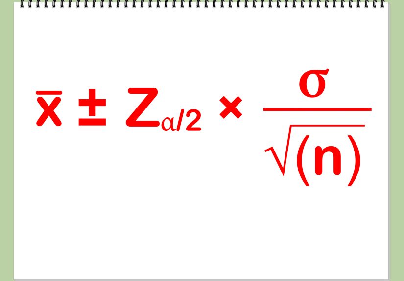
Mean, known population standard deviation:
x̄ ± z* (σ / √n)
Mean, unknown population standard deviation:
x̄ ± t* (s / √n)
Proportion:
p̂ ± z* √[ p̂(1 - p̂) / n ]
Final Thoughts
Learning how to calculate confidence interval values is one of those statistical skills that pays rent forever. Once you understand point estimate, standard error, critical value, and margin of error, the whole process becomes much less mysterious. You stop seeing the interval as a scary formula and start seeing it as a structured way to express uncertainty honestly.
That honesty is the real superpower. A confidence interval says, “Here is our best estimate, and here is how precise it seems to be.” In a world full of overconfident numbers, that is refreshing. Also, it keeps you from treating a sample result like a sacred prophecy carved into stone tablets by the gods of spreadsheet software.
Experience and Practical Lessons: What People Learn the Hard Way About Confidence Intervals
If you spend enough time around research reports, dashboards, product experiments, and survey results, you start to notice that confidence intervals are not difficult because the math is impossible. They are difficult because people are human. In practice, most mistakes happen long before the calculator comes out.
One common experience is that beginners fall in love with the point estimate and barely glance at the interval. A team sees a conversion rate of 8.4% and immediately starts celebrating, even though the confidence interval is wide enough to include outcomes that are merely average. That is the moment confidence intervals earn their keep. They force you to ask, “How sure are we, really?” which is not always the question the room wants to hear, but it is usually the one that matters.
Another lesson comes from sample size. People often expect a tiny sample to produce a polished, confident answer. Instead, they get a giant interval that looks like statistics shrugged and said, “Bring me more data.” That can feel annoying, but it is actually the method being honest. Wide intervals are not failures. They are warnings that the estimate is still unstable.
There is also a very practical workplace lesson: confidence intervals become easier when you write down your assumptions first. Are observations independent? Are you estimating a mean or a proportion? Do you know the population standard deviation? Is your sample large enough for the approximation you want to use? Five minutes of setup can save you from forty minutes of confident nonsense.
People also learn that interpretation is harder than calculation. Computing x̄ ± ME is often the easy part. Explaining what a 95% confidence interval actually means without slipping into incorrect wording is where many smart people suddenly look like they are assembling furniture without the instructions. The safest habit is to say the method is designed so that, over many repeated samples, 95% of such intervals would contain the true parameter. It is less catchy than saying “there is a 95% chance,” but it is more accurate.
Finally, real experience teaches that confidence intervals make conversations better. They lower the temperature. They replace fake certainty with useful boundaries. Instead of arguing whether a result is “real,” teams can discuss whether the plausible range is practically meaningful. That is a much better question. So yes, confidence intervals involve formulas, square roots, and critical values. But their real job is communication. They help you say, with a straight face and proper humility, “Here is what the data suggests, and here is how much trust we should place in it.”