How to Unhide Rows and Columns in Excel: 3 Quick Methods

Hidden rows and columns in Excel are a little like socks in a dryer: you know they were there a minute ago, but suddenly they have vanished into spreadsheet mythology. One moment your worksheet looks normal, and the next moment column D is missing, row 12 has gone undercover, and your carefully built report looks like it has been edited by a raccoon with a keyboard.

The good news? Learning how to unhide rows and columns in Excel is easy once you know where Excel hides the magic buttons. Whether you are working in Microsoft Excel for Microsoft 365, Excel 2021, Excel 2019, Excel 2016, Excel for Mac, or Excel for the web, the basic idea is the same: select the area around the hidden row or column, then tell Excel to show it again.

In this guide, you will learn three quick methods to unhide rows and columns in Excel, including the right-click method, the Ribbon method, and keyboard shortcuts. You will also learn how to unhide the first row or first column, how to reveal everything at once, and what to do when the usual Unhide command seems to be taking a coffee break.

Why Rows and Columns Get Hidden in Excel

Before we start clicking buttons with heroic confidence, it helps to know why rows and columns disappear in the first place. In most cases, Excel rows or columns are hidden intentionally. Someone may hide extra calculations, old notes, helper columns, sensitive information, unused sections, or messy data that does not need to appear in a printed report.

Hidden rows and columns are different from deleted rows and columns. If a row is deleted, the data is gone unless you undo the action or restore an earlier version. If a row is hidden, the data is still there. Excel is simply not showing it. Think of hiding as putting data behind a curtain, not throwing it into the recycling bin.

You can usually spot hidden rows or hidden columns by looking for gaps in the row numbers or column letters. For example, if your worksheet jumps from row 7 to row 10, rows 8 and 9 are probably hidden. If your columns jump from B to F, then columns C, D, and E are likely hiding somewhere between them, wearing tiny spreadsheet sunglasses.

Method 1: Unhide Rows and Columns with Right-Click

The right-click method is the fastest and friendliest way to unhide specific rows or columns in Excel. It works especially well when you already know exactly where the hidden area is located.

How to Unhide Hidden Rows with Right-Click

Suppose rows 5 through 8 are hidden. You can tell because the row numbers jump from 4 to 9. To unhide those rows, select the visible row above and the visible row below the hidden section. In this example, you would select rows 4 and 9.

After selecting the surrounding row headers, right-click one of the selected row numbers and choose Unhide. Excel will reveal the hidden rows between them. The missing data should return instantly, unless Excel has other settings involved, such as filters or very small row heights. We will deal with those sneaky gremlins later.

How to Unhide Hidden Columns with Right-Click

The process for columns is almost identical. If column C is hidden, select columns B and D. Then right-click one of the selected column letters and choose Unhide. Excel will display the hidden column between them.

This method is great for everyday fixes because it is visual and direct. You do not need to remember a shortcut or dig through the Ribbon. Just select around the missing area, right-click, and invite the hidden data back to the party.

Example: Unhiding a Missing Sales Column

Imagine you are reviewing a monthly sales worksheet. The columns are labeled Region, January, February, April, and May. Wait a minute. Where did March go? Unless your company has invented a new calendar, March is probably hidden.

To fix it, select the February and April column headers, right-click the selected area, and choose Unhide. Column March should reappear. Your sales report is now less suspicious, and your calendar can stop crying quietly in the corner.

Method 2: Use the Home Tab and Format Menu

The Ribbon method is another reliable way to unhide rows and columns in Excel. It is slightly less speedy than right-clicking, but it is excellent when you want a menu-based option that feels official, organized, and less like you are negotiating with the mouse.

How to Unhide Rows from the Ribbon

To unhide rows using the Excel Ribbon, first select the rows surrounding the hidden rows. Then go to the Home tab. In the Cells group, click Format. Under Visibility, point to Hide & Unhide, then select Unhide Rows.

This tells Excel to reveal hidden rows inside your selection. If you selected the entire worksheet, Excel will attempt to unhide all hidden rows on the sheet.

How to Unhide Columns from the Ribbon

To unhide columns, select the columns surrounding the hidden columns. Then go to Home, click Format, choose Hide & Unhide, and select Unhide Columns.

The Ribbon method is especially helpful for beginners because the command labels are clear. You can see exactly what Excel is about to do. It is also useful if your right-click menu is not appearing correctly or if you are working on a device where right-clicking feels awkward.

How to Unhide All Rows and Columns at Once

Sometimes you do not want to play detective. You do not want to inspect every row number, squint at every column letter, and whisper, “Where are you hiding, little spreadsheet goblin?” You just want everything visible again.

To unhide all rows and columns in Excel, select the entire worksheet. You can do this by clicking the small triangle in the top-left corner of the sheet, where the row numbers and column letters meet. You can also press Ctrl + A on Windows or Command + A on Mac. If your cursor is inside a data range, you may need to press the shortcut twice to select the whole sheet.

Once the entire sheet is selected, go to Home > Format > Hide & Unhide. Choose Unhide Rows, then repeat the same path and choose Unhide Columns. Excel will display hidden rows and columns across the worksheet, assuming they are truly hidden and not blocked by filters, grouping, protection, or tiny row heights.

Method 3: Use Keyboard Shortcuts for Speed

If you work in Excel often, keyboard shortcuts can save a surprising amount of time. They also make you look extremely efficient, which is nice if someone is watching over your shoulder and you want to give off “spreadsheet wizard” energy.

Shortcut to Unhide Rows in Excel

On Windows, select the rows around the hidden rows, then press Ctrl + Shift + 9. This shortcut unhides rows within the current selection.

For example, if rows 6 through 10 are hidden, select rows 5 and 11, then press Ctrl + Shift + 9. Excel should reveal the hidden rows. You can also select the entire worksheet first if you want to unhide all rows.

Shortcut to Unhide Columns in Excel

On Windows, the traditional shortcut for unhiding columns is Ctrl + Shift + 0. Select the columns around the hidden columns, then press the shortcut. For example, if columns C through E are hidden, select columns B and F, then press Ctrl + Shift + 0.

However, there is a small catch. On some Windows systems, Ctrl + Shift + 0 may be assigned to a language or keyboard setting, so it may not work until that system shortcut is changed. If the shortcut does nothing, do not panic. Excel is not judging you. Use the right-click method or the Ribbon method instead.

Mac Shortcut Notes

On Mac, Excel shortcuts can vary slightly depending on the keyboard, Excel version, and system settings. Many users rely on menu commands from the Ribbon or top menu because they are consistent. If you prefer shortcuts, check the current Excel keyboard shortcut list for your version and test them on a simple worksheet before using them in an important file.

How to Unhide the First Row or First Column in Excel

Unhiding the first row or first column can be trickier because there is no row above row 1 and no column to the left of column A. You cannot select the surrounding headers in the usual way because one side of the selection is missing. Excel, always dramatic, makes this feel harder than it needs to be.

Unhide Row 1

To unhide the first row, click in the Name Box, which is the small box to the left of the formula bar. Type A1 and press Enter. This selects cell A1, even if row 1 is hidden. Then go to Home > Format > Hide & Unhide > Unhide Rows.

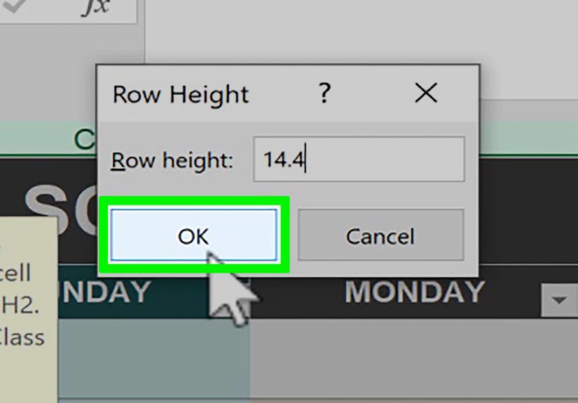
If that does not work, select the entire sheet, then use Home > Format > Row Height and enter a normal value, such as 15. Sometimes a row looks hidden because its height has been reduced to zero or nearly zero.

Unhide Column A

To unhide column A, use the Name Box again. Type A1 and press Enter. Then go to Home > Format > Hide & Unhide > Unhide Columns.

Another option is to select the entire sheet and adjust the column width. Go to Home > Format > Column Width and enter a standard width, such as 8.43. If column A was not technically hidden but had a tiny width, this will bring it back into view.

How to Tell If Rows Are Hidden or Filtered

One common Excel confusion is the difference between hidden rows and filtered rows. Both can make data disappear, but they are controlled in different ways.

Hidden rows are manually hidden by a user or macro. Filtered rows are temporarily hidden because a filter is showing only records that match specific criteria. For example, if a filter shows only sales from Texas, all other state rows may disappear from view. They are not manually hidden; they are filtered out.

To check for filters, look at the column headers. If you see filter arrows, a filter may be active. Go to the Data tab and choose Clear in the Sort & Filter group. This removes active filters and can instantly bring back rows that looked hidden.

Another clue is the row numbers. In some versions of Excel, filtered row numbers may appear in a different color or skip in a way that looks similar to hidden rows. If Unhide does not work, checking filters should be one of your first troubleshooting steps.

Why Unhide Might Not Work

Most of the time, the three methods above work perfectly. But occasionally Excel refuses to cooperate, because apparently even spreadsheets need a little drama. If your rows or columns still do not appear, here are the most likely reasons.

1. The Row Height or Column Width Is Too Small

A row can appear hidden if its height is set to zero or a very small number. A column can appear hidden if its width is reduced to almost nothing. In that case, the Unhide command may not behave the way you expect.

Select the entire worksheet, then go to Home > Format > Row Height and enter a normal value, such as 15. For columns, go to Home > Format > Column Width and enter a standard width, such as 8.43. This often restores rows or columns that seem impossible to unhide.

2. Filters Are Active

If filters are hiding rows, the Unhide command may not reveal them. Go to Data > Clear to remove active filters. You can also turn filters off completely by clicking Filter on the Data tab.

3. The Worksheet Is Protected

If the sheet is protected, you may not be allowed to unhide rows or columns. Go to the Review tab and look for Unprotect Sheet. If a password is required, you will need permission from the person who protected the workbook.

4. Rows or Columns Are Grouped

Excel has a grouping feature that lets users collapse and expand sections of a worksheet. If rows or columns are grouped, you may see small plus and minus buttons near the row numbers or column letters. Click the plus sign to expand the group.

You can also go to the Data tab and look in the Outline group. If the sheet uses grouping, the hidden sections may not be hidden in the ordinary sense. They may simply be collapsed.

5. Freeze Panes Makes the Sheet Look Strange

Freeze Panes does not hide rows or columns, but it can make navigation confusing. If the worksheet feels like parts of it are stuck in place, go to View > Freeze Panes > Unfreeze Panes. Then check whether the missing row or column is actually hidden.

Best Practices for Hiding and Unhiding Excel Data

Hiding rows and columns is useful, but it should not become a secret maze. If you share spreadsheets with coworkers, clients, teachers, or teammates, make your hidden sections easy to understand. Use clear labels, comments, or a small note explaining what has been hidden and why.

Avoid hiding critical data without telling the next person who will use the file. Hidden formulas, helper columns, or source data can cause confusion, especially when someone audits the workbook or tries to update a report. Excel files already have enough ways to surprise people. No need to add booby traps.

If you need to simplify a worksheet for presentation, consider grouping rows and columns instead of hiding them manually. Grouping provides visible expand and collapse buttons, which makes the worksheet easier to navigate. It also tells other users, “Hey, there is more information here,” instead of quietly burying data under the spreadsheet floorboards.

Quick Comparison of the 3 Methods

Right-Click Method

Best for quickly unhiding one specific row or column. Select the visible rows or columns around the hidden area, right-click, and choose Unhide.

Ribbon Method

Best for users who prefer menus or need a reliable option across different Excel versions. Use Home > Format > Hide & Unhide, then choose either Unhide Rows or Unhide Columns.

Keyboard Shortcut Method

Best for frequent Excel users who want speed. Use Ctrl + Shift + 9 to unhide rows. Use Ctrl + Shift + 0 to unhide columns on Windows, keeping in mind that system keyboard settings may interfere with the column shortcut.

Real-World Experience: What Unhiding Rows and Columns Teaches You

After working with enough spreadsheets, you learn that hidden rows and columns are not just a technical feature. They are a tiny window into how people think, organize, panic, and occasionally commit spreadsheet crimes against clarity. One workbook hides helper columns neatly and labels them like a responsible adult. Another hides half the data model with no explanation, as if future users are supposed to solve a financial escape room.

One practical lesson is to check for hidden rows and columns before making decisions from a worksheet. This is especially important in budgets, sales reports, grade trackers, inventory sheets, project plans, and exported data. A hidden column might contain formulas that explain the final numbers. A hidden row might include an adjustment, subtotal, or note that changes the meaning of the report. When something feels off, look for skipped row numbers or missing column letters before assuming the file is broken.

Another lesson is that unhiding everything can be safer than guessing. If you receive a workbook from someone else, selecting the whole sheet and using the Ribbon to unhide rows and columns can reveal whether any data was tucked away. This is not about being suspicious. It is about being thorough. Excel does not always announce, “By the way, some important stuff is hidden behind column G.” You have to check.

I have also learned that filters are responsible for many false alarms. People often say, “My rows are hidden and they will not unhide,” when the real issue is an active filter. The fix is usually simple: go to the Data tab and clear the filter. Suddenly, the missing rows return, and everyone pretends they were calm the whole time.

Column width and row height are another sneaky problem. A column with a width close to zero can look hidden, even if Excel does not treat it exactly like a normally hidden column. The same goes for rows with tiny heights. When Unhide does not work, resetting row height and column width is a practical next step. It is not glamorous, but neither is crawling under a desk to fix a loose cable, and that still saves the day.

The best experience-based advice is simple: hide data only when it improves the worksheet. Do not hide rows and columns just to make a messy workbook look clean. A clean-looking workbook with hidden chaos is still chaos; it is just wearing a nicer jacket. Use hidden rows and columns for supporting calculations, optional details, temporary views, or presentation cleanup. For anything important, document what you did.

If you are building a spreadsheet for other people, consider using color-coded helper columns, grouping, separate tabs, or clearly labeled sections instead of hiding everything. If you must hide rows or columns, add a note near the top of the sheet that says something like, “Some helper columns are hidden for readability.” Future users will appreciate it. Future you will appreciate it even more, especially three months later when you reopen the file and have absolutely no memory of your own cleverness.

Finally, make a habit of saving a backup before doing big cleanups. Unhiding rows and columns is usually safe, but if you are editing a shared workbook, a financial model, or a complicated report, backups are cheap insurance. Excel is powerful, but one enthusiastic round of clicking can still turn a beautiful workbook into a digital lasagna.

Conclusion

Knowing how to unhide rows and columns in Excel is one of those simple skills that saves time, prevents mistakes, and makes spreadsheets much less mysterious. The fastest method is usually right-clicking the surrounding row or column headers and choosing Unhide. The most beginner-friendly method is using Home > Format > Hide & Unhide. The speediest method for regular users is the keyboard shortcut approach.

If the hidden data still does not appear, check for filters, grouping, protected sheets, frozen panes, and tiny row heights or column widths. In Excel, missing data is not always missing. Sometimes it is just hiding behind a menu command, waiting for you to say the magic word: Unhide.

Note: This article is based on widely used Excel features and current guidance for Microsoft Excel versions commonly used in the United States, including Excel for Microsoft 365, Excel 2021, Excel 2019, Excel 2016, Excel for Mac, and Excel for the web. Menu names may vary slightly by version and device.